Research
5,000× Faster Thermal Simulations for 3D ICs
How LayerTherm combines physics, foundation models and heat-flow refinement for fast thermal feedback.
Thermal simulation is time-consuming: 10,000 cases at 30 minutes each would take 5,000 hours of serial computation, before parallelization or reuse.
Neural models can predict temperatures faster, but generalizing to new designs remains a challenge for approaches such as ThermFM (published in May 2026).
LayerTherm combines learned temperature patterns with heat-flow equations to handle new designs without fitting a new model for each one.
On ten public benchmark power maps, LayerTherm achieved approximately 5,000× speedup compared with the published Cadence Celsius runtime, with a 0.009 K mean temperature difference.
Unless explicitly attributed to a publication, the LayerTherm measurements and model comparisons below are Archgen Labs experiments reported in this research note, not results from the cited papers.
Thermal simulation takes time, and chip designers need to run it repeatedly. Each workload, layout or cooling change can produce a different temperature map. At 30 minutes per run, 10,000 evaluations would take 5,000 hours if run sequentially. Parallel execution and reuse reduce that time, but getting thermal feedback early remains difficult.
Conventional tools such as Celsius divide the chip and package into small regions and solve the heat-flow equations between them. Neural models can learn to approximate these solutions much faster:
- Poseidon demonstrated this approach for partial differential equations.
- ThermFM, whose extended paper appeared in May 2026, applies it to chip temperatures. But its published workflow uses solved temperature examples to fine-tune the model for a new chip. That adds both simulation time and model-training time before predictions can be used on that design.
Archgen Labs built LayerTherm to predict temperatures on new designs without that retraining step. It uses the design’s physical properties to estimate the temperature level, a neural model to predict the temperature pattern, and heat-flow equations to refine the result. We tested the same trained model on 85 unseen layouts without additional neural training.
LayerTherm architecture
LayerTherm divides the calculation into three layers.
- Physics layer: uses the new design’s power, materials, geometry and cooling to calculate the baseline temperature of each die: its average, one flat value per die.
- Foundational Model layer: takes the power map and finds the hotspots by predicting how much hotter or cooler each region runs than that baseline.
- Multivariate Function Solver (MVFS) layer: takes the combined estimate, the power map and the thermal conductances, checks that the heat generated matches the heat flowing out, and corrects the map until the mismatch is below the chosen tolerance.
- Input
- Physics
- Foundational Model
- MVFS
- Output
Layer 1: Physics sets each die’s baseline temperature
The physics layer works out how hot each die runs on average.
- Power tells us how much heat each die generates.
- Layer thicknesses, materials, interfaces and cooling tell us how easily that heat can leave.
- Fourier’s law, the basic law of heat conduction, says heat flows from hot to cold at a rate set by the material’s conductivity. Applied to a stack of layers, each layer acts as a resistor to heat flow, as in an electrical circuit.
Each layer: R = t / (k × A) · Each cooled face: R = 1 / (h × A)
Die average: Tdie = Tambient + P × (Rup × Rdown) / (Rup + Rdown)
q is heat flow per unit area, k thermal conductivity, ∇T the temperature gradient, t layer thickness, A die area, h the heat-transfer coefficient of the cooling, and P the die’s power. Rup and Rdown add up the layer resistances on the path to the heat sink above and to the board below; heat leaves through both paths in parallel. The full calculation solves the same chain of resistances layer by layer.
This sets each die’s baseline temperature, but not where the hotspots are.
- The result is one average temperature per die, taken from the design’s own physical description.
- It cannot locate local hot and cool regions; that is the next layer’s job.
The average-temperature calculation assumes layers that are uniform across the die, insulated die sides and uniform cooling over each face.
Layer 2: The Foundational Model finds the hotspots
The Foundational Model predicts how temperature varies around each die’s average, not the temperature itself.
- We remove the average from each power map, so the model sees where power is above or below average.
- It predicts the matching temperature pattern. A hotspot is learned as “this much hotter than the die average”.
- The physics layer sets the level, and a physically calibrated scale sets how large the pattern should be.
On a new layout, the model is used as is.
- We train it once, jointly across the training designs, so it sees varied patterns during training.
- On a new layout its weights stay fixed. The scale is calibrated from the layout’s geometry and synthetic power maps; no solved temperatures for that layout are needed.
The base model: DPOT-S
- DPOT (Denoising Operator Transformer) is an open-source neural operator from Tsinghua University’s machine-learning group, published at ICML 2024. The code and pretrained weights are at github.com/thu-ml/DPOT.
- It was pretrained on a mix of public simulation datasets (FNO data, PDEBench, PDEArena and CFDBench), so it has already seen many kinds of physical fields.
- It mixes information across the whole map with Fourier-based layers. We fine-tuned DPOT-S, with 30.8 million parameters, using the same recipe as for Poseidon.
- LayerTherm uses DPOT-S because it gave the better final result: on the 85 unseen layouts, the full pipeline built on DPOT-S reached a mean error of 5.56 × 10⁻⁵ K, against 5.98 × 10⁻⁵ K with Poseidon-T.
- Appendix A compares the two. The 85-layout figures in the Accuracy section were measured with the earlier Poseidon-T version.
Layer 3: MVFS corrects the map
MVFS checks the estimate against the laws of heat flow and fixes what is left.
- It divides the stack into small cells and checks, cell by cell, whether the heat generated matches the heat flowing out.
- Where they do not match, it adjusts the temperatures and checks again, until the remaining mismatch is below the selected tolerance.
G × correction = r
Final temperature = initial temperature + correction
G describes how easily heat flows between neighboring cells and out through the cooling boundaries. r is the mismatch: the heat that the current estimate does not account for.
This is still a thermal calculation, but a much smaller one.
- It starts from the combined physics and model estimate and refines it, rather than repeating a complete commercial meshing and simulation workflow.
- It needs no reference temperature map and does not retrain the model.
Accuracy breakdown
To measure error, we need trusted reference temperatures to compare against.
- Both LayerTherm and ThermFM produce temperature maps. To know how good a prediction is, we need the correct answer for the same layout and power.
- For that we use PACT, the open-source Parallel Compact Thermal simulator. It is a conventional thermal solver that supports IC designs from single chips to 3D stacks.
- PACT solves the full heat-flow equations for each layout. We treat its result as the correct answer and report every error against it.
- PACT is open source; reproducing our exact reference temperatures also requires the layout and power inputs, material and boundary-condition settings, solver version, and run configuration.
The 85 test layouts are real placed designs that neither model saw during training.
- They include arithmetic, signal-processing, memory and interconnect IPs, as well as CPU and accelerator designs.
- Their size ranges from roughly 15,000 to 2 million cell instances.
- Each layout is a two-die stack with 30 power scenarios, taken from simulated switching activity: 2,550 scenarios in total.
After all three layers, LayerTherm’s error is about 220,000 times smaller than our Therm-FM implementation’s in this zero-adaptation test.
- Average error (mean RMSE): 5.98 × 10⁻⁵ K for LayerTherm, against 13.29 K for ThermFM.
- Peak-temperature error: 1.28 × 10⁻⁴ K, against 14.47 K.
Both approaches were tested without any training on the target layouts.
- ThermFM here is our own jointly trained implementation of the ThermFM approach.
- This is a test of transfer without adaptation, not the fine-tuned setting reported in the ThermFM paper.
| 85 unseen layouts · 2,550 scenarios | Mean RMSE | Peak-temperature error |
|---|---|---|
| ThermFM | 13.29 K | 14.47 K |
| LayerTherm | 5.98 × 10⁻⁵ K | 1.28 × 10⁻⁴ K |
The same model weights were used across all 85 test layouts.
- New layouts still require their physical system to be set up.
- Changes to the material stack, TSV arrangement or cooling require an accurate physical description and validation.
All 2,550 scenarios met the selected relative residual threshold of 0.001. The layouts share a reference stack and cooling setup; their median within-map temperature spread is 7.5 × 10⁻³ K. A three-layout control found that the Foundational Model’s starting field used the same or more refinement iterations than a flat physical baseline. Learning improved the initial pattern; an additional refinement-speed benefit was not demonstrated.
Comparison with Celsius
We also compared LayerTherm with Cadence Celsius on a public benchmark.
- We used all ten released power maps from the DeepOHeat paper’s public Celsius benchmark (full reference): one 1 × 1 × 0.5 mm block with different surface-power patterns.1
- The table reports measured LayerTherm results on a GCP CPU VM, using 32,000 thermal cells.
| Power map | Published Celsius time | LayerTherm time | Mean difference | Largest point difference | Timing ratio |
|---|---|---|---|---|---|
| map_5_5 | About 5 min | 66.79 ms | 0.00379 K | 0.11057 K | ≈4,492× |
| map_10_10 | About 5 min | 67.14 ms | 0.00824 K | 0.10812 K | ≈4,468× |
| map_20_20 | About 5 min | 31.48 ms | 0.00439 K | 0.01300 K | ≈9,530× |
| map_c1 | About 5 min | 65.41 ms | 0.00850 K | 0.14489 K | ≈4,586× |
| map_c2 | About 5 min | 67.34 ms | 0.00948 K | 0.09244 K | ≈4,455× |
| map_c3 | About 5 min | 65.83 ms | 0.00985 K | 0.15918 K | ≈4,557× |
| map_c4 | About 5 min | 66.40 ms | 0.01343 K | 0.13405 K | ≈4,518× |
| map_c5 | About 5 min | 66.05 ms | 0.01170 K | 0.14036 K | ≈4,542× |
| map_c6 | About 5 min | 66.38 ms | 0.01295 K | 0.25199 K | ≈4,519× |
| map_c7 | About 5 min | 67.24 ms | 0.00595 K | 0.17893 K | ≈4,462× |
| Overall | About 5 min | 66.39 ms median | 0.00883 K | 0.25199 K maximum | ≈5,013× mean ratio |
Mean timing ratio = average of (300,000 ms ÷ each map’s time): 5,013×. The ratio at the median time of 66.39 ms is 4,519×; these are different summaries.
Public benchmark designs
We also ran LayerTherm on nine public, open-source designs, from about 15,000 to 1.6 million cell instances, and compared it with PACT.
- The designs are seven RISC-V processors (Ibex, TinyRocket, SweRV, CVA6, Ariane133, Black Parrot and BP Quad) and two tensor accelerators (TPU and OpenTPU). None of them is among the 85 test layouts.
- Eight ship as example designs with the OpenROAD flow scripts; OpenTPU is the open-source OpenTPU accelerator, laid out with the same flow. Ariane133 and Black Parrot are also part of the ChiPBench chip-placement benchmark, and BP Quad is a TILOS MacroPlacement test case.
| Design | Cell instances | PACT s | LayerTherm ms | Speedup | RMSE K | Peak-temp. error K |
|---|---|---|---|---|---|---|
| Ibex | 15,196 | 8.824 | 136.2 | ≈65× | 0.00047 | 0.00047 |
| TinyRocket | 29,692 | 8.617 | 126.7 | ≈68× | 0.001731 | 0.001052 |
| TPU | 51,165 | 8.974 | 129.5 | ≈69× | 0.000966 | 0.001826 |
| SweRV | 97,386 | 9.126 | 116.0 | ≈79× | 0.00776 | 0.003245 |
| CVA6 | 121,086 | 7.929 | 142.3 | ≈56× | 0.002307 | 0.004132 |
| Ariane133 | 167,855 | 121.651 | 308.4 | ≈394× | 0.012565 | 0.016016 |
| Black Parrot | 219,191 | 119.770 | 307.9 | ≈389× | 0.003599 | 0.007103 |
| OpenTPU | 404,965 | 134.155 | 126.7 | ≈1,059× | 0.002818 | 0.005191 |
| BP Quad | 1,566,090 | 298.565 | 306.9 | ≈973× | 0.063825 | 0.106761 |
| Overall | 15k–1.6M | 9.126 median | 136.2 median | ≈350× mean ratio | 0.010671 mean | 0.106761 maximum |
RMSE and peak-temperature error are measured against PACT. They are temperature differences, so the values are the same in K and °C. In the Overall row, times are medians, the speedup is the average of the nine per-design ratios, RMSE is the mean over the nine designs and the peak-temperature error is the largest.
What the results show:
- LayerTherm took 116–308 ms per design, against 7.9–299 s for PACT: between 56× and 1,059× faster.
- The gap is widest on the larger designs: on the four above 160,000 instances, LayerTherm was 389× to 1,059× faster.
- RMSE stayed below 0.07 K on every design, and below 0.013 K on all but BP Quad. The largest peak-temperature error was 0.107 K, also on BP Quad.
PACT and LayerTherm side by side
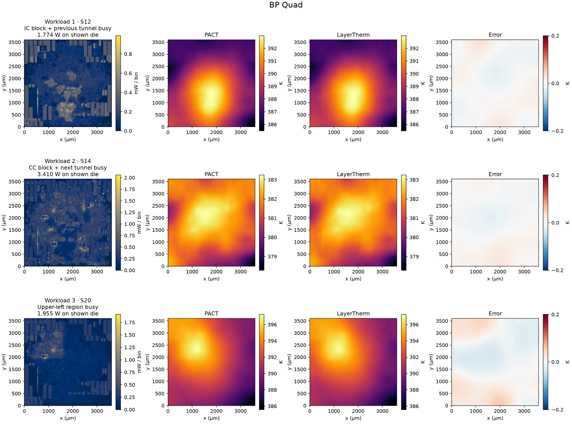
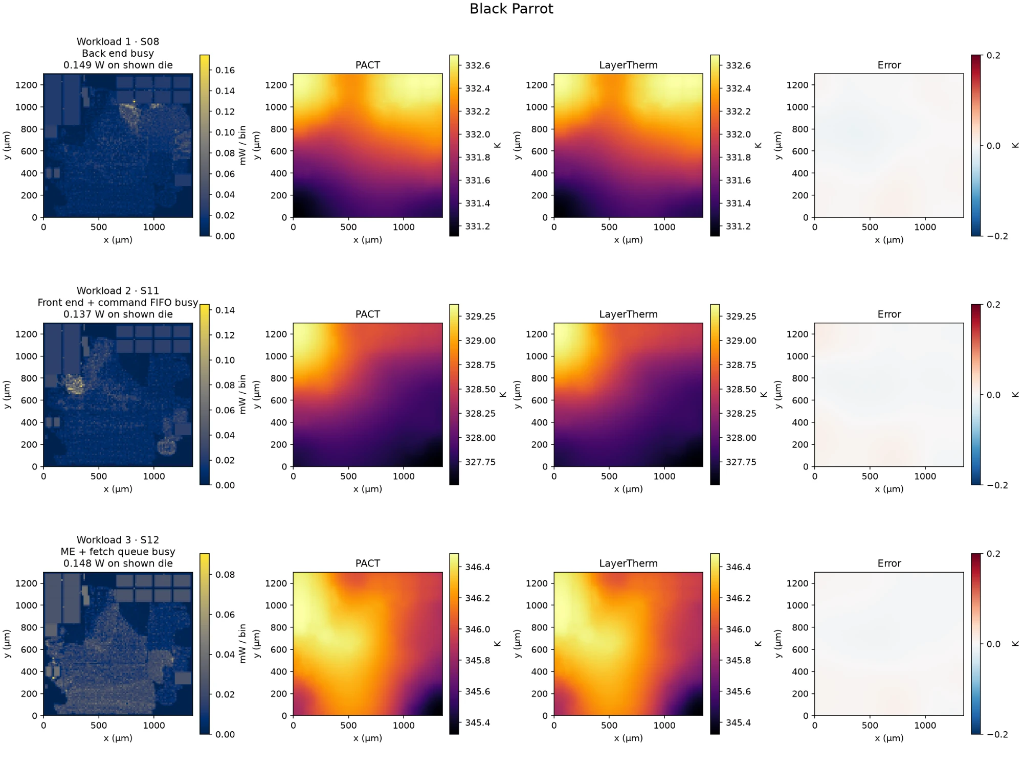
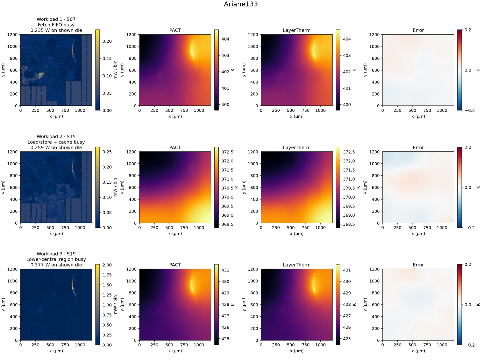
The figures show three workloads each for the three largest processors.
- BP Quad: a four-core BlackParrot RISC-V processor, and the largest design (1,566,090 cell instances, 220 macros).
- Black Parrot: a single 64-bit BlackParrot RISC-V core with a cache-coherence directory (219,191 cell instances, 24 macros).
- Ariane133: the 64-bit Ariane RISC-V core, now called CVA6, laid out with 132 memory macros (167,855 cell instances). It is a different configuration from the CVA6 row in the table.
- In every row the LayerTherm map is hard to tell apart from PACT, and the error stays well inside the ±0.2 K color scale.
What LayerTherm delivers
1. Faster thermal feedback
LayerTherm returns temperatures in milliseconds, and its lead over a conventional solver is largest on the biggest designs.
- On the ten public Celsius power maps: 31–67 ms, against a published Celsius runtime of about five minutes (roughly 5,000×).
- On the nine public designs: 116–308 ms, against 7.9–299 s for PACT (56× to 1,059×).
- In our scaling tests, a conventional direct solver’s time grew almost with the square of the number of thermal cells, while LayerTherm’s grew roughly in proportion.
2. Better accuracy on unseen layouts
On 85 layouts it had never seen, LayerTherm’s average error is about 220,000 times smaller than our Therm-FM implementation’s in this zero-adaptation test.
- Every one of the 85 layouts finished below 6 × 10⁻⁴ K average error.
- On the nine public designs, RMSE against PACT stayed below 0.07 K.
- Separating the physical level from the learned pattern fixed the transfer error, and MVFS removed what was left.
3. Reuse without retraining
One trained Foundational Model served all 85 new layouts, with no retraining for any of them.
- Illustrative data-generation cost. A workflow requiring 5,000–10,000 solves at an assumed 30 minutes each would take approximately 104–208 days serially, before parallelization or reuse. This is not a universal requirement or Therm-FM’s reported sample count: Therm-FM reports cross-chip adaptation using 10–30 target samples in some experiments.
- LayerTherm skips that step. A new design supplies its physical description, and MVFS checks the result against the heat-flow equations: all 2,550 scenarios passed that check.
- Our own model training (10.8 hours on one GPU for DPOT-S) happened once and is not repeated for new designs.
Working on a chiplet or 3D stack? Tell us where thermal checks slow your design loop.
Write to hari@archgen.tech or naveen@archgen.tech to discuss LayerTherm for your design.
Appendix A: Foundation models for thermal simulation
We began with an open-source foundation model and asked two questions.
- Can it capture small hot regions accurately?
- Can the same trained model work on layouts it has never seen?
We chose the base model first, then improved the training objective, then changed what the model was asked to learn.
Choosing the base model
We first built the Foundational Model on Poseidon-T, an open-source foundation model for physics simulations.
- Poseidon was built by ETH Zurich and pretrained on a large set of fluid-flow simulations, so it has already learned how smooth physical fields behave.
- The version we use has about 21 million parameters. It reads a map in small local windows (an attention-based U-Net design).
- We fine-tune it on our training designs, rather than training a model from scratch.
In a head-to-head test against DPOT-S, Poseidon’s raw predictions transferred better to new layouts.
- DPOT-S is a different open foundation model: a Fourier-based transformer pretrained on a different set of simulations.
- We trained it with exactly the same data, recipe and training budget, then compared the two models on their own.
| Same recipe, two base models | Poseidon-T | DPOT-S used in LayerTherm |
|---|---|---|
| Design | Attention-based U-Net (Swin-V2) | Fourier-based transformer (AFNO) |
| Pretrained on | Fluid-flow simulations | A mix of public PDE simulation datasets |
| Size | ~21 M parameters | 30.8 M parameters |
| Training time, same GPU | 5.2 h | 10.8 h |
| Validation error on the training designs relative, lower is better | 0.000190 | 0.000204 |
| More accurate prediction on new layouts share of 2,550 scenarios | 89.6% | 10.4% |
What the comparison shows:
- On the designs they were trained on, the two models were equally accurate: their validation errors are about 7% apart.
- On new layouts, given the same physics input, Poseidon’s prediction was better in 89.6% of the 2,550 scenarios.
- Poseidon also trains in half the time.
- After the MVFS layer the order reverses: DPOT-S finishes with a mean error of 5.56 × 10⁻⁵ K, about 7% lower than the 5.98 × 10⁻⁵ K with Poseidon-T. That is why LayerTherm uses DPOT-S (see Layer 2).
One training run per model. DPOT-S used learning rates tuned for Poseidon, which may slightly disadvantage it; differences under about 20% should be read with that in mind.
Give hot regions more weight during training
A model can look accurate on average while still missing a small hotspot.
- A small hot region contributes little to an average error, so ordinary training can neglect it.
- We changed the training objective (the loss function) to give more weight to points where the reference temperature changes steeply, which is where hotspots sit:
wᵢ = (1 + αgᵢ) / mean(1 + αg)
Loss = mean[wᵢ × (predicted Tᵢ − reference Tᵢ)²]
Updating the loss function reduced the error at the hottest point for a single design, but it still did not generalize across designs.
- On one benchmark design, the error at the maximum point fell by about 7%, with no added cost at prediction time.
- On layouts the model had not seen, its errors stayed large. Better hotspot fitting did not solve the problem of moving to a new design.
Why the model did not transfer to new layouts
On layouts it had never seen, the model was off by more than 13 K on average.
- Trained on: our suite of designs, predicting absolute temperatures. The suite covers arithmetic, signal-processing, crypto, memory and interconnect IPs, as well as CPU and accelerator designs, from roughly 15,000 to 2 million cell instances.
- Tested on: 85 unseen layouts, with 30 power scenarios each (2,550 scenarios).
- Result: average error (RMSE) of 13.29 K, and 14.47 K error in peak temperature.
The model was being asked to solve two different problems at once.
- The overall temperature level. How hot a die runs on average depends mainly on its package and cooling: how much heat goes in and how easily it gets out. That changes from one design to the next.
- The pattern around that level. Where the hotter and cooler regions sit depends mainly on where power is used on the die.
- The model had to learn both from the training designs. On a new layout with a different package, it got the overall level wrong, which shifted the whole temperature map up or down.
- Training on more designs did not fix this. Asking one network to learn both the level and the pattern was making transfer harder.
So we split the work: physics sets the level, and the model learns only the pattern.
1. DeepOHeat, DAC 2023, published Celsius runtime and reference benchmark; released inputs and reference fields. The approximately five-minute figure is a reported single-simulation timing, not ten independently published per-map timings. Ratios use the published Xeon runtime and measured GCP CPU request times, excluding setup and I/O, rather than a matched-hardware rerun. A physics-only control achieved the same accuracy in 59.34 ms; these results do not establish an incremental neural speed benefit.
References
- Zhen Huang et al. Therm-FM: Foundation Model is ALL YOU NEED for 3D-ICs Thermal Simulation. arXiv:2605.22663, 2026. Code and models. Our zero-adaptation comparison is distinct from the paper’s adapted-model evaluation.
- Maximilian Herde et al. Poseidon: Efficient Foundation Models for PDEs. NeurIPS 2024. Code.
- DeepOHeat — Celsius benchmark source. Ziyue Liu et al. DeepOHeat: Operator Learning-based Ultra-fast Thermal Simulation in 3D-IC Design. DAC 2023. Released benchmark and code. The Celsius timing used here is published reference timing, not a matched-hardware rerun.
- Zhongkai Hao et al. DPOT: Auto-Regressive Denoising Operator Transformer for Large-Scale PDE Pre-Training. 2024. Code and pretrained models.
- PACT: Parallel Compact Thermal simulator. Reference solver used in the Archgen experiments.
- OpenROAD flow scripts. Source of the public example-design flow used in the benchmark.
- Zhihai Wang et al. Benchmarking End-To-End Performance of AI-Based Chip Placement Algorithms. 2024. Introduces ChiPBench.
- TILOS MacroPlacement. Source of the BP Quad benchmark context.